Grouping and Hiding Data in Excel – how to use both of these features in your spreadsheets
![]() This week’s hint and tip is on grouping and hiding data in Excel. Both grouping and hiding are ways in which you can alter how your data appears in your spreadsheets. We cover this area of data displaying in our Basic Excel training course but decided to do a hint and tip on it too. We are going to go through it now below.
This week’s hint and tip is on grouping and hiding data in Excel. Both grouping and hiding are ways in which you can alter how your data appears in your spreadsheets. We cover this area of data displaying in our Basic Excel training course but decided to do a hint and tip on it too. We are going to go through it now below.
There are a number of ways in which you can alter how your data is displayed in Excel, two of these being grouping and hiding. Both of these options allow you to ‘remove’ your data out of view on your screen.
Grouping Data
Grouping data in Excel is a useful way to organise and summarise data, especially when dealing with large spreadsheets of data. It allows you to temporarily ‘hide’ your data by using the option to expand or collapse the outline that is created through using the group option. This outline is shown as a plus or minus symbol on the left hand side of the spreadsheet.
You can find this option on the Data Tab, either as a visible ‘Group’ button on the ribbon or by clicking the ‘Outline’ button, which reveals the ‘Group’ button in a small dropdown ribbon. You can use this option to group together both rows and columns.

To group data together, you select the rows that you want to temporarily hide underneath the ‘heading’ row or column. From here you then go to the Data Tab and click on the Group option. This will have now created the outline on the left hand side, shown by a plus or a minus. Clicking on this allows you to expand and collapse the data.
So in the example in the video below, we grouped all the individual food items under the food heading row. This allows you to collapse to just see the total numbers for each food category or expand to see all the individual numbers as well as the total.

Hiding Data
Hiding rows and columns in Excel is a simple way to keep your data organized and make your spreadsheet easier to read. This option completely hides the rows or columns from your view.

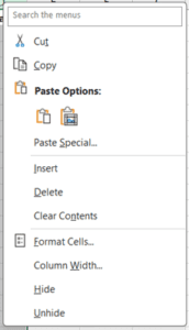
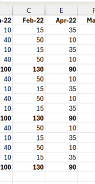
To Hide a column or columns, simply select the column headings at the top of the worksheet. From here right click on the column heading and select the option Hide. To reverse simply highlight the columns either side of the hidden ones and right hand click on a column heading and select unhide.

The video below shows you how you can use this feature, we hope that you find it useful and enjoy learning about it!
Take a look below at the video to find out more and then try it out on your own computer!
We hope you have enjoyed this hint and tip on grouping and hiding data in Excel. Why not take a look at our previous video hint and tip on how to create a calculated field in Excel for a Pivot Table?
