
Creating a Calculated Field in a Pivot Table in Excel – how to create these in your Pivot Tables in your spreadsheets
![]() This week’s hint and tip is on creating a calculated field in Excel. Calculated fields are an option that you can use when you are creating Pivot Tables in your spreadsheets in Excel. We cover Pivot Tables and the fields you use in our Advanced Excel training course but not creating a calculated field. As this isn’t specifically covered in our course, we decided to do a hint and tip on it. We are going to go through it now below.
This week’s hint and tip is on creating a calculated field in Excel. Calculated fields are an option that you can use when you are creating Pivot Tables in your spreadsheets in Excel. We cover Pivot Tables and the fields you use in our Advanced Excel training course but not creating a calculated field. As this isn’t specifically covered in our course, we decided to do a hint and tip on it. We are going to go through it now below.
What is a calculated field?
A calculated field is a formula that calculates something using one or more fields normally in your Pivot Table. These are normally used if the summaries produced in the Pivot Table are not exactly what you want. These calculated fields enable you to create your own formulas or calculations to give the results you are looking for.
Creating a calculated field
We are going to look at how to create a simple calculated field in an Excel Pivot Table. Once created you can then use it as a field in the Pivot Table just like any other field. It does not appear on the data transactional sheet from which the Pivot Table was first created, simply as a new calculated field on the pivot table.
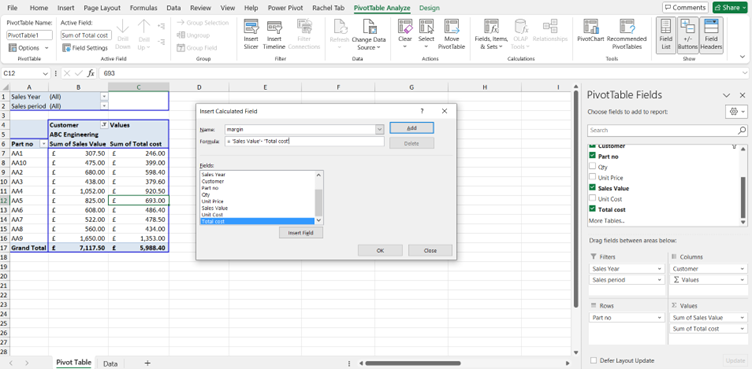
The screenshot below shows a basic Pivot Table on the left and a pop up window next to it. To get this pop up window, you click on the ‘Fields, Items and Sets’ button on the PivotTable Analyze Tab. From the list that appears after clicking on this button, select the ‘Calculated Field’ option. This will then give you the pop up window. This will now let you create your calculated field.
You will need to type in the Name for your new field and then the formula for it. In the example, Margin has been chosen as the name and then =Sales value-Total Cost for the formula. You build up the formula by double clicking on those fields. Once you have filled this all in, click on Add. This will add the calculated field to the list of fields available.
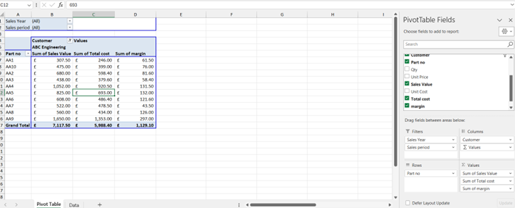
Now that the calculated field has been created, you can add it to your pivot table from the list of available fields. As shown below, the field is added into the ‘Values’ area which has inserted it into the Pivot Table as shown. On the right hand side you can see the new field in the values quadrant of the Pivot Table fields list.
Video with example spreadsheet
The video below shows you how you can use this feature in the spreadsheet attached here. (clicking here will download a copy to your computer so you can try it out!). We hope that you find the video useful and enjoy learning about it!
Take a look below at the video to find out more and then try it out on your own computer!
We hope you have enjoyed this hint and tip on creating a calculated field in Excel. Why not take a look at our previous video hint and tip on how to insert a hierarchy SmartArt diagram in a PowerPoint presentation?