UNIQUE Function in Excel – another way of filtering out data in your spreadsheets

UNIQUE Function in Excel – have you used this function before to filter out data in your spreadsheets?

This week’s hint and tip is on the UNIQUE Function in Excel. Functions, also known as formulas, are used by many people in Excel on a daily basis. We have previously looked at different ways to filter in Excel through the more standard routes that most have heard of. The UNIQUE function gives another way in which you can filter out data in your spreadsheet. We cover a lot of functions in our courses but we don’t cover the UNIQUE one specifically so decided to do a hint and tip on it. We are going to go through it now below.

The UNIQUE Function

The UNIQUE function works in a similar way to Advanced Filtering on the Data Tab but with another variant as you will see below and in the video we have produced.

The layout of this function is: =UNIQUE(Array,By_col,Exactly_once)

This function has 3 parts (or arguments) to it which are talked through more in the video below:

1. Array: the range of cells in which you want to return unique rows or columns from
2. By_col: you either type in FALSE or TRUE
   • FALSE – to return the unique rows
   • TRUE – to return the unique columns
3. Exactly_once: you either type in FALSE or TRUE
   • FALSE – to return rows or columns that only occur once in the array
   • TRUE – to return all the unique rows or columns that occur in the range

As there are multiple arguments in this function there is more than one variation that you can use in your spreadsheets. We are gong to look at 2 examples in this hint and tip below.

Variant 1

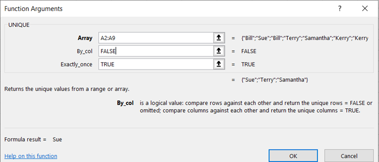
The first variation is to use UNIQUE to select from an array of data in a column the unique rows where they only appear once.

Variant 2

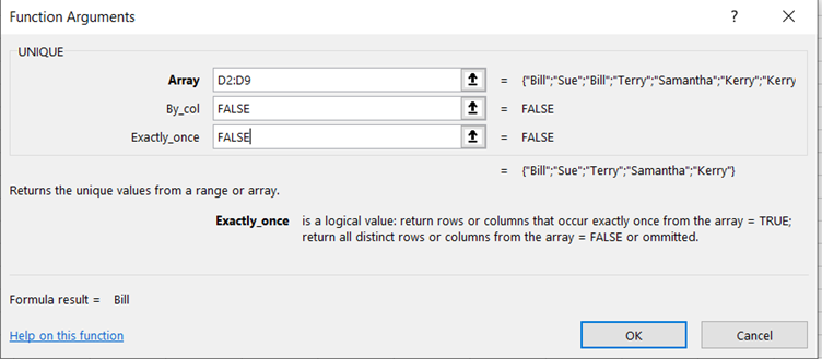
The second variation is to use UNIQUE to select from an array of data in a column all the unique rows not just those appearing once.

The video below goes through how to use this function in the spreadsheet attached here (clicking here will download a copy to your computer so you can try it out!). We hope that you find the video useful and enjoy learning about it!

Take a look below at the video to find out more!

We hope you liked this hint and tip on the UNIQUE Function in Excel, why not take a look at our previous one on using the automatic updating feature of Styles in Word?